Voronoi Diagrams on a Spherical Surface
- class voronoi_utility.Voronoi_Sphere_Surface(points, sphere_radius=None, sphere_center_origin_offset_vector=None)[source]
Voronoi diagrams on the surface of a sphere.
Parameters: points : array, shape (npoints, 3)
Coordinates of points used to construct a Voronoi diagram on the surface of a sphere.
sphere_radius : float
Radius of the sphere (providing radius is more accurate than forcing an estimate). Default: None (force estimation).
sphere_center_origin_offset_vector : array, shape (3,)
A 1D numpy array that can be subtracted from the generators (original data points) to translate the center of the sphere back to the origin. Default: None assumes already centered at origin.
Notes
Note that, at the moment, the code is using a pure planar surface area calculation instead of performing the spherical surface area calculation described below. This is because of the buggy behaviour of the spherical polygon surface area code and the generally more robust performance of the planar code for a wide variety of test cases. The accuracy of the planar surface area calculations will depend on the density of generators – a high density should generally perform much better than a low density. Basically, it will be important to monitor the extent of reconstitution for specific cases when using the code in its current state.
The algorithm depends on the important realization that the convex hull of the generators on the sphere surface is equivalent to the Delaunay triangulation [Caroli]. The Delaunay facet normals are then equivalent to the Voronoi vertices on the surface of the sphere [Fortune]. The fact that each Voronoi vertex is equidistant to at least three generators can be used to build an appropriate data structure associating Voronoi vertices with their contained generator.
The calculation of surface areas for the Voronoi regions currently appears to be susceptible to numerical instabilities, which may in part relate to arc cosine operations. For example, sphere radii of 1.9999 or 87.0 are pathological test cases but radii of 2.0 or 1.1 are tolerated. In theory, the surface area of a spherical polygon can be calculated using the following equation [Weisstein]:
\[S = [\theta - (n-2) \pi]R^2\]Where \(\theta\) is the sum of the inner angles of the polygon, \(R\) is sphere radius, and \(n\) is the number of polygon vertices. Unfortunately, as n approaches a large number of vertices and / or in the presence of nearly-coplanar vertices, the equation is susceptible to producing invalid areas \(\le 0\). In such cases, the algorithm falls back to a conventional surface area calculation for a planar polygon, as an approximation.
References
[Caroli] (1, 2) Caroli et al. (2009) INRIA 7004 [Fortune] (1, 2) Fortune, S. http://www.qhull.org/html/qdelaun.htm [Weisstein] (1, 2) Weisstein, Eric W. “Spherical Polygon.” From MathWorld–A Wolfram Web Resource. http://mathworld.wolfram.com/SphericalPolygon.html Examples
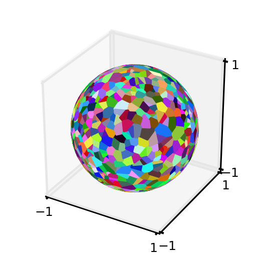
Produce a Voronoi diagram for a pseudo-random set of points on the unit sphere:
>>> import matplotlib
>>> import matplotlib.pyplot as plt
>>> import matplotlib.colors as colors
>>> from mpl_toolkits.mplot3d import Axes3D
>>> from mpl_toolkits.mplot3d.art3d import Poly3DCollection
>>> import numpy as np
>>> import scipy as sp
>>> import voronoi_utility
>>> #pin down the pseudo random number generator (prng) object to avoid certain pathological generator sets
>>> prng = np.random.RandomState(117) #otherwise, would need to filter the random data to ensure Voronoi diagram is possible
>>> #produce 1000 random points on the unit sphere using the above seed
>>> random_coordinate_array = voronoi_utility.generate_random_array_spherical_generators(1000,1.0,prng)
>>> #produce the Voronoi diagram data
>>> voronoi_instance = voronoi_utility.Voronoi_Sphere_Surface(random_coordinate_array,1.0)
>>> dictionary_voronoi_polygon_vertices = voronoi_instance.voronoi_region_vertices_spherical_surface()
>>> #plot the Voronoi diagram
>>> fig = plt.figure()
>>> fig.set_size_inches(2,2)
>>> ax = fig.add_subplot(111, projection='3d')
>>> for generator_index, voronoi_region in dictionary_voronoi_polygon_vertices.iteritems():
...    random_color = colors.rgb2hex(sp.rand(3))
...    #fill in the Voronoi region (polygon) that contains the generator:
...    polygon = Poly3DCollection([voronoi_region],alpha=1.0)
...    polygon.set_color(random_color)
...    ax.add_collection3d(polygon)
>>> ax.set_xlim(-1,1);ax.set_ylim(-1,1);ax.set_zlim(-1,1);
(-1, 1)
(-1, 1)
(-1, 1)
>>> ax.set_xticks([-1,1]);ax.set_yticks([-1,1]);ax.set_zticks([-1,1]);
[<matplotlib.axis.XTick object at 0x...>, <matplotlib.axis.XTick object at 0x...>]
[<matplotlib.axis.XTick object at 0x...>, <matplotlib.axis.XTick object at 0x...>]
[<matplotlib.axis.XTick object at 0x...>, <matplotlib.axis.XTick object at 0x...>]
>>> plt.tick_params(axis='both', which='major', labelsize=6)
Now, calculate the surface areas of the Voronoi region polygons and verify that the reconstituted surface area is sensible:
>>> import math
>>> dictionary_voronoi_polygon_surface_areas = voronoi_instance.voronoi_region_surface_areas_spherical_surface()
>>> theoretical_surface_area_unit_sphere = 4 * math.pi
>>> reconstituted_surface_area_Voronoi_regions = sum(dictionary_voronoi_polygon_surface_areas.itervalues())
>>> percent_area_recovery = round((reconstituted_surface_area_Voronoi_regions / theoretical_surface_area_unit_sphere) * 100., 5)
>>> print percent_area_recovery
97.87551
>>> #that seems reasonable for now
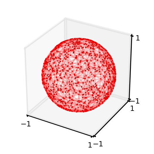
For completeness, produce the Delaunay triangulation on the surface of the unit sphere for the same data set:
>>> Delaunay_triangles = voronoi_instance.delaunay_triangulation_spherical_surface()
>>> fig2 = plt.figure()
>>> fig2.set_size_inches(2,2)
>>> ax = fig2.add_subplot(111, projection='3d')
>>> for triangle_coordinate_array in Delaunay_triangles:
...     m = ax.plot(triangle_coordinate_array[...,0],triangle_coordinate_array[...,1],triangle_coordinate_array[...,2],c='r',alpha=0.1)
...     connecting_array = np.delete(triangle_coordinate_array,1,0)
...     n = ax.plot(connecting_array[...,0],connecting_array[...,1],connecting_array[...,2],c='r',alpha=0.1)
>>> o = ax.scatter(random_coordinate_array[...,0],random_coordinate_array[...,1],random_coordinate_array[...,2],c='k',lw=0,s=0.9)
>>> ax.set_xlim(-1,1);ax.set_ylim(-1,1);ax.set_zlim(-1,1);
(-1, 1)
(-1, 1)
(-1, 1)
>>> ax.set_xticks([-1,1]);ax.set_yticks([-1,1]);ax.set_zticks([-1,1]);
[<matplotlib.axis.XTick object at 0x...>, <matplotlib.axis.XTick object at 0x...>]
[<matplotlib.axis.XTick object at 0x...>, <matplotlib.axis.XTick object at 0x...>]
[<matplotlib.axis.XTick object at 0x...>, <matplotlib.axis.XTick object at 0x...>]
>>> plt.tick_params(axis='both', which='major', labelsize=6)
Methods
- delaunay_triangulation_spherical_surface()[source]
Delaunay tessellation of the points on the surface of the sphere. This is simply the 3D convex hull of the points. Returns a shape (N,3,3) array of points representing the vertices of the Delaunay triangulation on the sphere (i.e., N three-dimensional triangle vertex arrays).
- voronoi_region_surface_areas_spherical_surface()[source]
Returns a dictionary with the estimated surface areas of the Voronoi region polygons corresponding to each generator (original data point) index. Attempts to calculate the spherical surface area but falls back to a planar estimate if the spherical excess is <= 0. An example dictionary entry: {generator_index : surface_area, ...}.
- voronoi_region_vertices_spherical_surface()[source]
Returns a dictionary with the sorted (non-intersecting) polygon vertices for the Voronoi regions associated with each generator (original data point) index. A dictionary entry would be structured as follows: {generator_index : array_polygon_vertices, ...}.